In the previous two sessions, we introduced Pandas’ data structures and common calculation methods. Time series analysis is a crucial data processing approach in the field of geoscience.
By understanding the temporal variation characteristics of data, we can gain deeper insights into the evolutionary patterns and physical mechanisms of the subjects under study.
Therefore, this session explores some common methods for handling time series data in geoscience from the perspective of time series data processing in Pandas.
Timestamp
A string or encoded information representing a specific point in time. It typically consists of a set of numbers representing the amount of time elapsed from a reference point (e.g., Greenwich Mean Time January 1, 1970, 00:00:00 UTC), in units of seconds or milliseconds.In Python, the
timeanddatetimemodules can be used to handle timestamps. Since these functionalities are built into the Pandas module, we don’t need to use the aforementioned modules separately.
Creating Time Series
There are primarily two ways to create time series in Pandas:
- Create a time series using the built-in
date_rangefunction in Pandas. This function can specify parameters like start date, end date, time step, etc., and returns aDatetimeIndexobject. - Convert date-time strings in other formats to a
DatetimeIndexobject using Pandas’to_datetimefunction (very useful when we need to convert date columns read into Pandas tables to time format).
The following examples illustrate the use of these two methods.
Creating Time Series with date_range
The date_range function can create continuous time series in various forms by combining different parameters. We first generate a time series by specifying start and end times and a time step (freq).
Common time steps (freq) in Pandas include:
S: SecondT: MinuteH: HourD: DayB: Business day (weekday)W: WeekM: Month (end)Q: Quarter (end)Y: Year (end)
We can prefix the time step with a number to customize it, e.g., 2H for 2 hours.
python
import pandas as pd

# Known start and end dates, generate date series, default step is 1 day.
date_range = pd.date_range(start='2021-01-01', end='2021-01-04')
print(date_range)

date_range = pd.date_range(start='2021-01-01', end='2021-05-07', freq='M')          # Set step to month (end)
print(date_range)

date_range = pd.date_range(start='2021-01-01', end='2021-08-07', freq='3M')         # Set step to 3 months
print(date_range)

date_range = pd.date_range(start='2021-01-01', end='2021-05-07', freq='5W')          # Set step to week
print(date_range)

date_range = pd.date_range(start='2021-01-01', end='2021-01-06', freq='B')          # Set step to business day
print(date_range)

date_range = pd.date_range(start='2021-01-01', end='2021-11-07', freq='Q')          # Set step to quarter (end)
print(date_range)

date_range = pd.date_range(start='2021-01-01', end='2023-05-07', freq='YS')          # Set step to year (start)
print(date_range)

# Output:
# DatetimeIndex(['2021-01-01', '2021-01-02', '2021-01-03', '2021-01-04'], dtype='datetime64[ns]', freq='D')
# DatetimeIndex(['2021-01-31', '2021-02-28', '2021-03-31', '2021-04-30'], dtype='datetime64[ns]', freq='M')
# DatetimeIndex(['2021-01-31', '2021-04-30', '2021-07-31'], dtype='datetime64[ns]', freq='3M')
# DatetimeIndex(['2021-01-03', '2021-02-07', '2021-03-14', '2021-04-18'], dtype='datetime64[ns]', freq='5W-SUN')
# DatetimeIndex(['2021-01-01', '2021-01-04', '2021-01-05', '2021-01-06'], dtype='datetime64[ns]', freq='B')
# DatetimeIndex(['2021-03-31', '2021-06-30', '2021-09-30'], dtype='datetime64[ns]', freq='Q-DEC')
# DatetimeIndex(['2021-01-01', '2022-01-01', '2023-01-01'], dtype='datetime64[ns]', freq='AS-JAN')
We can notice that dates generated by weekly, monthly, and quarterly steps default to the last day. Also, the quarterly calculation by default follows natural seasons (e.g., March-April-May as the first quarter).
We can perform some customizations:
python
date_range = pd.date_range(start='2021-01-01', end='2021-04-07', freq='MS')         # Set generated date to the first day of the month, MS (month start)
print(date_range)

date_range = pd.date_range(start='2021-01-01', end='2021-05-07', freq='QS')         # Set generated date to the first day of the quarter, with quarter start month changed to January.
print(date_range)

date_range = pd.date_range(start='2021-01-01', end='2024-05-07', freq='YS')         # Set generated date to the first day of the year.
print(date_range)

date_range = pd.date_range(start='2021-01-01', end='2021-01-15', freq='W-MON')      # Set generated date to Mondays of each week.
print(date_range)

date_range = pd.date_range(start='2023-01-01', end='2024-01-15', freq='QS-FEB')     # Set generated date to the first day of the quarter, starting with February.
print(date_range)

# Output:
# DatetimeIndex(['2021-01-01', '2021-02-01', '2021-03-01', '2021-04-01'], dtype='datetime64[ns]', freq='MS')
# DatetimeIndex(['2021-01-01', '2021-04-01'], dtype='datetime64[ns]', freq='QS-JAN')
# DatetimeIndex(['2021-01-01', '2022-01-01', '2023-01-01', '2024-01-01'], dtype='datetime64[ns]', freq='AS-JAN')
# DatetimeIndex(['2021-01-04', '2021-01-11'], dtype='datetime64[ns]', freq='W-MON')
# DatetimeIndex(['2023-02-01', '2023-05-01', '2023-08-01', '2023-11-01'], dtype='datetime64[ns]', freq='QS-FEB')
In some cases, we only know the initial date or the end date. We can calculate the time series by specifying the desired time step and number of periods.
python
date_range = pd.date_range(start='2021-01-01', freq='D', periods=7)         # Known start date, frequency, number of periods.
print(date_range)

date_range = pd.date_range(end='2021-01-07', freq='W', periods=7)           # Known end date, frequency, number of periods.
print(date_range)

# Output:
# DatetimeIndex(['2021-01-01', '2021-01-02', '2021-01-03', '2021-01-04',
#                '2021-01-05', '2021-01-06', '2021-01-07'],
#               dtype='datetime64[ns]', freq='D')
# DatetimeIndex(['2020-11-22', '2020-11-29', '2020-12-06', '2020-12-13',
#                '2020-12-20', '2020-12-27', '2021-01-03'],
#               dtype='datetime64[ns]', freq='W-SUN')
Additionally, the date_range function includes several potentially useful parameters:
tz: Specifies the time zone. Default isNone, meaning use the system default time zone.normalize: Normalize dates to 00:00. Default isFalse.name: Specifies the name for the generated time series.inclusive: In older versions, this wasclosed. Determines whether the generated date range includes the start and end dates. Default is'left'(left-closed, right-open). Other options are'right'(left-open, right-closed),'both'(left-closed, right-closed),'neither'(left-open, right-open).
python
date_range = pd.date_range('2021-01-01', '2021-01-05', freq='D', tz='Asia/Tokyo')           # Tokyo time (UTC+9)
print(date_range)
print(date_range.tz_convert('UTC'))             # Convert to UTC

# Output:
# DatetimeIndex(['2021-01-01 00:00:00+09:00', '2021-01-02 00:00:00+09:00',
#                '2021-01-03 00:00:00+09:00', '2021-01-04 00:00:00+09:00',
#                '2021-01-05 00:00:00+09:00'],
#               dtype='datetime64[ns, Asia/Tokyo]', freq='D')
# DatetimeIndex(['2020-12-31 15:00:00+00:00', '2021-01-01 15:00:00+00:00',
#                '2021-01-02 15:00:00+00:00', '2021-01-03 15:00:00+00:00',
#                '2021-01-04 15:00:00+00:00'],
#               dtype='datetime64[ns, UTC]', freq='D')

date_range = pd.date_range('2021-01-01 12:25:56', '2021-12-31', freq='M')
print(date_range[0])
date_range = pd.date_range('2021-01-01 12:25:56', '2021-12-31', freq='M', normalize=True)       # Normalize date to 00:00:00
print(date_range[0])

# Output:
# 2021-01-31 12:25:56
# 2021-01-31 00:00:00

date_range = pd.date_range('2021-01-01', '2021-12-31', freq='Q', name='Seasonal')
print(date_range)

date_range = pd.date_range('2024-05-01', '2024-05-04', inclusive='left')
print(date_range)
date_range = pd.date_range('2024-05-01', '2024-05-04', inclusive='right')
print(date_range)
date_range = pd.date_range('2024-05-01', '2024-05-04', inclusive='both')
print(date_range)
date_range = pd.date_range('2024-05-01', '2024-05-04', inclusive='neither')
print(date_range)

# Output:
# DatetimeIndex(['2021-03-31', '2021-06-30', '2021-09-30', '2021-12-31'], dtype='datetime64[ns]', name='Seasonal', freq='Q-DEC')
# DatetimeIndex(['2024-05-01', '2024-05-02', '2024-05-03'], dtype='datetime64[ns]', freq='D')
# DatetimeIndex(['2024-05-02', '2024-05-03', '2024-05-04'], dtype='datetime64[ns]', freq='D')
# DatetimeIndex(['2024-05-01', '2024-05-02', '2024-05-03', '2024-05-04'], dtype='datetime64[ns]', freq='D')
# DatetimeIndex(['2024-05-02', '2024-05-03'], dtype='datetime64[ns]', freq='D')
Creating Time Series from Other Formats
“Other formats” generally refer to date-time in string form, like '2021-01-01'. When importing large amounts of time-stamped data from external files, we can conveniently convert it to a time series using the to_datetime function.
Let’s read a .csv file from an external source and convert its date-time column to a time series.
python
pth = r'F:\Proj_Geoscience.Philosophy\Material\tmp_SSP2.csv'

df = pd.read_csv(pth, index_col=0)
print(df.head()) # Display first few rows

# Output example (assuming temperature data):
#             ACCESS-CM2  EC-Earth3  EC-Earth3-Veg  MPI-ESM1-2-HR  GFDL-ESM4  \
# 1990-12-31   -9.838771  -9.637003      -9.321887     -10.383628  -9.549001
# 1991-12-31  -10.165740  -9.453364      -9.650858     -10.076542  -9.783594
# 1992-12-31  -10.944804 -10.569817      -9.624666     -10.221733  -9.442735
# 1993-12-31  -11.011893 -10.919116      -9.689930     -10.822980  -9.617322
# 1994-12-31   -9.935500  -9.687431     -10.403852     -10.077468  -9.583637
# ...                ...        ...            ...            ...        ...
# [111 rows x 7 columns]
Here, we read a temperature data file using Pandas’
read_csvfunction. The first row by default becomes the DataFrame column names. Since we specified the parameterindex_col=0, the first column is set as the row index (row names).
Now, let’s convert the DataFrame’s index from strings to date format.
python
print(df.index)
df.index = pd.to_datetime(df.index)
print(df.index)

# Output:
# Index(['1990-12-31', '1991-12-31', '1992-12-31', '1993-12-31', '1994-12-31',
#        '1995-12-31', '1996-12-31', '1997-12-31', '1998-12-31', '1999-12-31',
#        ...
#        '2091-12-31', '2092-12-31', '2093-12-31', '2094-12-31', '2095-12-31',
#        '2096-12-31', '2097-12-31', '2098-12-31', '2099-12-31', '2100-12-31'],
#       dtype='object', length=111)
# DatetimeIndex(['1990-12-31', '1991-12-31', '1992-12-31', '1993-12-31',
#                '1994-12-31', '1995-12-31', '1996-12-31', '1997-12-31',
#                '1998-12-31', '1999-12-31',
#                ...
#                '2091-12-31', '2092-12-31', '2093-12-31', '2094-12-31',
#                '2095-12-31', '2096-12-31', '2097-12-31', '2098-12-31',
#                '2099-12-31', '2100-12-31'],
#               dtype='datetime64[ns]', length=111, freq=None)
We can also directly convert strings, lists, etc., not necessarily only Pandas objects.
python
print(pd.to_datetime('2021-01'))
print(pd.to_datetime(['2021-01-01', '2021-01-02']))

# Output:
# 2021-01-01 00:00:00
# DatetimeIndex(['2021-01-01', '2021-01-02'], dtype='datetime64[ns]', freq=None)
In the to_datetime function, the format parameter can specify the date format, e.g., %Y-%m-%d for year-month-day. For unconventional date formats, we can define custom date formats for parsing and conversion.
Here, year, month, day, hour, minute, second are represented by %Y, %m, %d, %H, %M, %S respectively.
python
print(pd.to_datetime('202101', format='%Y%m'))          # Direct parsing will cause an error, so we need to specify the date format.
print(pd.to_datetime(['20211', '20212', '202112'], format='%Y%m'))

# Output:
# 2021-01-01 00:00:00
# DatetimeIndex(['2021-01-01', '2021-02-01', '2021-12-01'], dtype='datetime64[ns]', freq=None)
Shifting Time Series
In some cases, there may be misalignment issues with multi-source time series, requiring time series shifting. Pandas provides several methods for shifting time series.
python
date_range = pd.date_range('2021-01-01', '2021-01-05', freq='D')
print(date_range)
print(date_range.shift(1))          # Shift based on the current step unit (freq).
print(date_range.shift(-3))
print(date_range.shift(2, freq='M'))    # Shift based on a specified step unit.
print(date_range + pd.offsets.Week(3))

# Generate time offsets.
dt = pd.to_timedelta(3, unit='D')
print(dt)
print(date_range + dt)

dt = pd.to_timedelta(['1 D', '2 H', '3 minutes', '4 seconds', '5 w'])
print(date_range + dt)

dt = pd.to_timedelta('5 days 7 hours 30 minutes 10 seconds')
print(date_range + dt)

# Output:
# DatetimeIndex(['2021-01-01', '2021-01-02', '2021-01-03', '2021-01-04',
#                '2021-01-05'],
#               dtype='datetime64[ns]', freq='D')
# DatetimeIndex(['2021-01-02', '2021-01-03', '2021-01-04', '2021-01-05',
#                '2021-01-06'],
#               dtype='datetime64[ns]', freq='D')
# DatetimeIndex(['2020-12-29', '2020-12-30', '2020-12-31', '2021-01-01',
#                '2021-01-02'],
#               dtype='datetime64[ns]', freq='D')
# DatetimeIndex(['2021-02-28', '2021-02-28', '2021-02-28', '2021-02-28',
#                '2021-02-28'],
#               dtype='datetime64[ns]', freq=None)
# DatetimeIndex(['2021-01-22', '2021-01-23', '2021-01-24', '2021-01-25',
#                '2021-01-26'],
#               dtype='datetime64[ns]', freq=None)
# 3 days 00:00:00
# DatetimeIndex(['2021-01-04', '2021-01-05', '2021-01-06', '2021-01-07',
#                '2021-01-08'],
#               dtype='datetime64[ns]', freq='D')
# DatetimeIndex(['2021-01-02 00:00:00', '2021-01-02 02:00:00',
#                '2021-01-03 00:03:00', '2021-01-04 00:00:04',
#                '2021-02-09 00:00:00'],
#               dtype='datetime64[ns]', freq=None)
# DatetimeIndex(['2021-01-06 07:30:10', '2021-01-07 07:30:10',
#                '2021-01-08 07:30:10', '2021-01-09 07:30:10',
#                '2021-01-10 07:30:10'],
#               dtype='datetime64[ns]', freq='D')
Time Series Data Processing
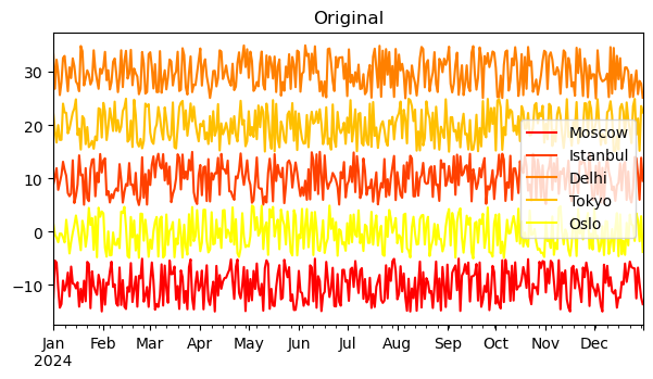
Due to the periodicity of time and inconsistent month lengths, time series data processing is more complex than simple algebraic operations. Let’s illustrate with a set of pseudo-meteorological data.
python
import numpy as np

# Generate a set of daily temperature data.
df_tmp = pd.DataFrame(index=pd.date_range('2024-01-01', '2024-12-31', freq='D'))
df_tmp['Moscow'] = np.random.rand(len(df_tmp)) * 10 - 15
df_tmp['Istanbul'] = np.random.rand(len(df_tmp)) * 10 + 5
df_tmp['Delhi'] = np.random.rand(len(df_tmp)) * 10 + 25
df_tmp['Tokyo'] = np.random.rand(len(df_tmp)) * 10 + 15
df_tmp['Oslo'] = np.random.rand(len(df_tmp)) * 10 - 5

print(df_tmp.head())

# Output (example):
#                Moscow   Istanbul      Delhi      Tokyo      Oslo
# 2024-01-01 -12.507333   8.843648  33.246008  22.083794  1.464828
# 2024-01-02  -5.420229  10.210387  26.832628  18.923657 -0.535928
# 2024-01-03  -5.777253  11.924500  32.288078  16.753620 -1.134632
# 2024-01-04 -10.513435   7.863196  29.965339  20.013110 -1.965073
# 2024-01-05 -14.257012   9.221470  25.657996  17.241110 -0.337181
# ...               ...        ...        ...        ...       ...
# [366 rows x 5 columns]

# Regular algebraic statistics.
print(df_tmp.mean())
print(df_tmp.min())
print(df_tmp.max())

# Output (example):
# Moscow      -10.028244
# Istanbul      9.980530
# Delhi        29.889565
# Tokyo        19.897225
# Oslo         -0.263960
# dtype: float64
# Moscow      -14.968037
# Istanbul      5.008738
# Delhi        25.021508
# Tokyo        15.016760
# Oslo         -4.997246
# dtype: float64
# Moscow       -5.049498
# Istanbul     14.995171
# Delhi        34.974616
# Tokyo        24.968358
# Oslo          4.908233
# dtype: float64
Long-term climatology is a significant aspect of geoscience. We can use the resample method to downsample daily-scale data to monthly, annual, quarterly, weekly, etc.
python
print(df_tmp.resample('M').mean())           # Monthly average temperature.
print(df_tmp.resample('QS-DEC').mean())      # Seasonal average temperature (seasons ending in Dec, Mar, Jun, Sep).

# Output (example):
#                Moscow   Istanbul      Delhi      Tokyo      Oslo
# 2024-01-31 -10.254586   9.863383  29.811591  19.542478  0.118495
# 2024-02-29 -10.574170   8.663596  29.921715  20.434315 -0.765250
# ...               ...        ...        ...        ...       ...
#                Moscow   Istanbul      Delhi      Tokyo      Oslo
# 2023-12-01 -10.409052   9.283486  29.864818  19.973533 -0.308648
# 2024-03-01 -10.080890  10.365666  29.859606  19.775936 -0.076268
# ...
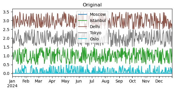
If the variable is precipitation, total precipitation might be more meaningful than average precipitation. In this case, the resampling aggregation function can be changed from mean to sum to calculate total precipitation.
python
df_prc = df_tmp.copy() / 10
df_prc[df_prc < 0] = 0 # Set negative values (unrealistic for precipitation) to 0.

print(df_prc.head())
print(df_prc.resample('Y').sum())       # Annual total precipitation.

# Output (example):
#            Moscow  Istanbul     Delhi     Tokyo      Oslo
# 2024-01-01     0.0  0.884365  3.324601  2.208379  0.146483
# 2024-01-02     0.0  1.021039  2.683263  1.892366  0.000000
# ...
#            Moscow    Istanbul        Delhi       Tokyo       Oslo
# 2024-12-31     0.0  365.287396  1093.958072  728.238447  41.132944
In commonly used ERA5 data, the provided monthly precipitation is often the daily average within the month. Regarding the issues of inconsistent month lengths and leap years, we can solve them simply using Pandas time series.
python
df_prc_month_day = pd.DataFrame(index=pd.date_range('2024-01-01', periods=12, freq='M'))
df_prc_month_day['Delhi'] = np.random.rand(df_prc_month_day.shape[0]) * 15
df_prc_month_day['Mumbai'] = np.random.rand(df_prc_month_day.shape[0]) * 15
df_prc_month_day['Bangalore'] = np.random.rand(df_prc_month_day.shape[0]) * 15
print(df_prc_month_day)

# Multiply by the number of days in each month to get monthly total.
print(df_prc_month_day.mul(df_prc_month_day.index.days_in_month, axis=0))

# Output (example):
#                 Delhi     Mumbai  Bangalore
# 2024-01-31   3.940283  14.243030  14.550210
# 2024-02-29  10.600057   3.372597  11.475781
# ...
#                   Delhi      Mumbai   Bangalore
# 2024-01-31  122.148777  441.533943  451.056512
# 2024-02-29  307.401667   97.805311  332.797655
# ...
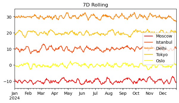
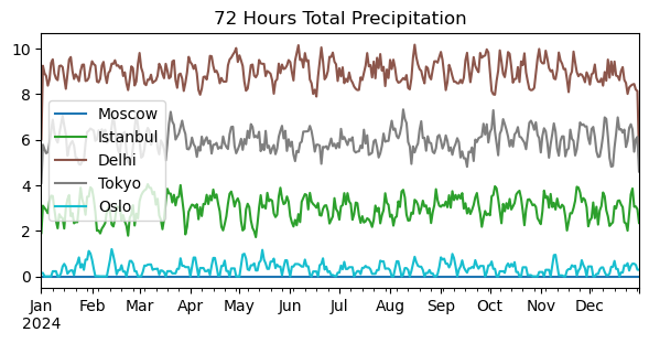
Given the instability of meteorological conditions, smoothing and denoising are commonly used methods. Or we might need to calculate metrics like three-day total precipitation, all requiring time series data processing. Below, we use a classic built-in method in Pandas — the sliding window method rolling — to implement filtering.
Common parameters for this function include:
window: The size of the sliding window. It’s often set to an odd number for symmetry on both ends.min_periods: The minimum number of observations within the window. If the count is less than this value, the result will be NaN.center: Whether to align the window’s center point to the middle of the original time series. Default isFalse(aligned to the right edge).axis: Specifies the axis for sliding. Default is0.
python
print(df_tmp.rolling(window=7).mean())                                       # 7-day moving average temperature.
print(df_tmp.rolling(window=7, center=True).mean())                          # Window center aligned.
print(df_tmp.rolling(window=7, min_periods=1, center=True).mean())           # Minimum window set to 1.

# Output (first few rows example):
#               Moscow   Istanbul      Delhi      Tokyo      Oslo
# 2024-01-01       NaN        NaN        NaN        NaN       NaN
# 2024-01-02       NaN        NaN        NaN        NaN       NaN
# ...
# (With center=True, min_periods=1, no NaNs at the start/end with proper padding.)

# Calculate 72-hour total precipitation (3-day sum).
print(df_prc.rolling(window=3, center=True, min_periods=1).sum())

# Output (example):
#            Moscow  Istanbul     Delhi     Tokyo      Oslo
# 2024-01-01     0.0  1.905404  6.007864  4.100745  0.146483
# 2024-01-02     0.0  3.097854  9.236671  5.776107  0.146483
# ...
Postscript
The above covers some introductions to handling time series data with Pandas. Richer and deeper usages are essentially combinations and extensions of these basics. We only need to master these fundamental components to achieve our ultimate goals through different assembly methods.
Undoubtedly, these contents are still quite introductory; more exploration is needed. Additionally, similar to date_range and to_datetime, there are period_range and to_period functions. Their usage is almost identical, but the latter emphasizes the concept of a period (a span of time).
However, generally, if we consider the step between two consecutive timestamps to be fixed, the concept of a period becomes less necessary. Therefore, this article won’t elaborate further (it’s already a long session, almost twice as long as I imagined!).